OK so you have encountered a lot about “RMS” in audio recording, mixing and mastering. You might have read it many times in different tutorials featured in this blog or in recording forums. So what is really RMS?
RMS is Root Mean Square
It is assumed you are not a mathematician or have strong engineering knowledge so let’s explain this term in the easiest way. RMS stands for Root mean square. Do not confuse with those squares or means; the easiest way to understand RMS is simply it’s just an unique way of finding out the “average”.
Why not simply use the word “average” instead of “RMS”? Well, technically RMS is used to characterize the “average” of continuous varying signals such as audio, electrical signals, sound, etc.
Like any properties of a continuous signal such as audio or electrical signals. It can be characterized as having a maximum, minimum and average. In audio waveforms, these maximum is often called “peak” signal and often measured in dB in digital. In digital audio, the maximum allowable is 0dB. If it exceeds that amount, distortion would occur.
Between the minimum (the quietest sections of the audio) and the loudest section (towards 0dBFS, the peak) is where the RMS value can be found. It would be depicted on the screenshot below:
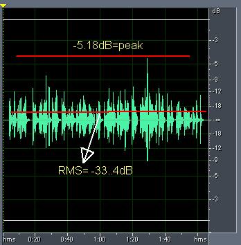
Now you can understand these terms very easily. The highest point of the waveform is called “peak”, the value shown is -5.18dB. The RMS is very far away down at -33.4dB.
The origin of RMS value in digital audio
As promised to you, there won’t be showcasing of complex mathematics behind RMS. But one thing worth observing on the above screenshot is that the RMS value seems to be found at location where most common signal levels are also found.
Since the RMS is at -33.4dB. This is also the “average” loudness of the waveform taking into account all “instances” of loudness statistics in the waveform.
To understand the computation graphically, let’s use a histogram which is a tool to show the distribution/occurrences of loudness throughout the waveform. See the histogram below:
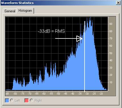
Interpreting the histogram, the RMS value is found in the most common loudness region of the waveform which is around -35dB to -25dB. However it’s computed to be -33dB and not -28dB where it has the highest number of occurrences as shown in the histogram; why?
The reason is that the loudness is skewed to your left and RMS takes consideration of all loudness data in the waveform. It is why the RMS is slightly skewed from -28dB to the actual value is -33.4dB.
Let’s present a normalized audio (where loud and quite sections are even, so it’s a highly compressed audio), and see where the RMS can be found. Take a look at the screenshot below:
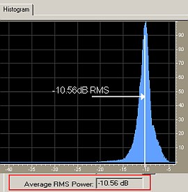
Since the entire audio is now balanced (not skewed), the RMS is found in the center and coincides exactly with the region of highest occurrences as shown in the histogram (which is -10.56dB).


One response
Hi Emerson, thanks for these great explanations about RMS ! I’m not in the audio domain but could easily understand what is it and how it’s used thanks to your article.