Audio Recording

How to View the Frequency Spectrum of an Audio Wave

If you are dealing with frequency analysis of the audio wave “quantitatively”, one of the best tools I have learned in my signals/engineering class is FFT or Fast Fourier Transform. It is an algorithm to compute the Fourier transform equivalent of a time domain. This highly advanced technique is very simple to understand, it simply converts a time domain function into a frequency domain function.

After audio mix down (where all sound of the instruments are cohesively combined into a single wave), the song is represented as a time domain function as we can see that the x – axis of the wave is using a time element in hours: minutes: seconds (only minutes and seconds is used realistically). See screen shot below:

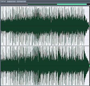
But time domain graph of the audio wave specially used during the mastering process of the track is simply a plot of amplitude (y-axis) versus time. Obviously you cannot see the frequencies of that wave. It is why we used FFT (Fast Fourier Transform) to convert this time domain representation into a frequency domain plot. With frequency domain, you can analyze the amplitude (y-axis) versus Frequencies.

Though, it is highly recommended to stick to your ear when working with commercial audio production however you can see a glimpse of the frequency response of the track. For example, if you like to check if the uppermost frequency ranges (20,000Hz) has been already filtered. It is very hard to detect it using a human ear. In this case, you need a spectrum plot.

Using Adobe Audition, you can open your wave in edit view, and then click “Analyze” –> Show frequency analysis –> Set the FFT size to a maximum, as this increases the resolution and accuracy of the frequency plot. Set the type to default (Blackmann – Harris) and there you can see the frequency response graph. See below:

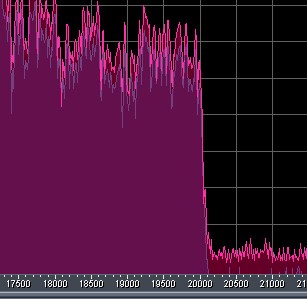
As you can see, it is confirmed that that a sharp low pass filter has been implemented with cutoff at 20,000 Hz (see plot above). This low pass filter can be implemented using Butter worth.

This is just an example of the wonderful application of FFT algorithm to see the Frequency spectrum. I won’t go into details as it becomes technically difficult to be understood by common readers; because of the extreme use of mathematics.

For students, please check this out:
Fast Fourier Transform Wiki notes
What is Fourier Transform?