
This is an introductory tutorial for beginners in digital audio waveform. This will give you the most important information necessary when working with digital audio regardless of what DAW (digital audio workstation) you are using and the type of projects you are doing. The digital audio waveform is an object that can be described by a lot of properties. As an audio engineer, you will be manipulating these properties in your project to get the sound you need. To manipulate these properties, you will be using a lot of tools such as compressor, parametric equalizer, sample rate converter etc. Let’s start, see an example waveform below:
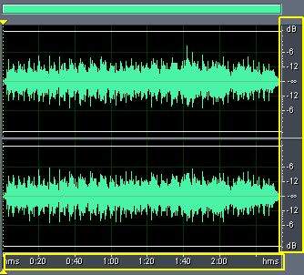
digital audio waveform
In most recording software, the default waveform is using amplitude vs. time representation of digital audio (also called the “time domain” representation). Take note the x and y-axis of the waveform (inside the yellow box). The following are the major visible waveform properties:
1.) Duration – shown in the x-axis of the waveform is the time property of the waveform. It tells the duration of the audio waveform (e.g. 2 minutes long).
2.) Amplitude – shown in the y-axis is the amplitude property of the waveform. Amplitude in digital audio is scaled in dBFS (logarithmic scale) which tells the loudness or the volume of the waveform at given time. dBFS means decibel “relative to full scale”. In digital audio, the maximum digital audio level is 0dBFS. Beyond this level, you increase the risk of clipping and distortion in your digital audio signal which will result to undesirable effects in audio quality. The y-axis is scaled from 0dBFS (maximum possible level) all the way down to negative infinity dB (flat line) which signifies complete audio silence. So this implies that -3dBFS is louder than -12dBFS or -12dBFS is louder than -36dBFS. Farther the value of the decibel below 0 dBFS; the lesser will be its resulting loudness.
3.) Number of channels – In the above screenshot, you see two waveforms in the time domain which means there are two channels in the waveform. Two channels mean it is a “stereo” audio waveform. In some waveforms, you can only see one waveform, and it is called a “mono” audio waveform. This is the most commonly used format in recording/tracking (e.g. guitars, vocals, drums, etc.). During audio mixing, you will be summing all mono tracks into a single stereo waveform for mastering. Also in multichannel projects, you will have more than 2 channels and it is called “surround” audio.
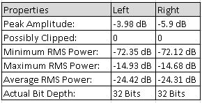
There are also non-visible digital audio waveform properties that are important. To know these properties, you need a tool that can provide the statistics of the waveform. This is usually available in most standard recording software. For example in Adobe Audition 1.5, you can get the waveform statistics by selecting the entire waveform first (pressing Control – A) then go to Analyze – Statistics. Below are the properties:
other properties of the digital audio
4.) Peak Amplitude – This is the maximum peak in the entire waveform (from beginning to end). For example in the above screenshot, there are two values -3.98 dBFS for left and -5.9 dBFS for right because the waveform is stereo (two-channels). Since the peak amplitude is less than 0dBFS there will be no clipped signal as confirmed by the statistics. Peak amplitude is very useful in recording and mixing digital audio. For example, an important recording clipping prevention technique in recording/tracking is to never exceed -6dBFS peak from start to end. This will ensure you have a lot of headroom in your digital audio which will also prevent distortion/clipping at the same time. In some recording sessions, this may increase to -3dBFS as long as no signal will peak at 0dBFS or more. During audio mixing, all tracks peak amplitude as well as the mix down should never exceed -3 dBFS in order to have correct audio mixing levels and headroom in preparation for mastering.
5.) Minimum RMS power – this is the lowest “RMS” volume detected on the waveform. Take note that this is not “peak” measurement but rather “RMS”.
6.) Maximum RMS power – the loudest RMS volume detected on the waveform.
7.) Average RMS power – this is the average perceived loudness of the entire waveform. This is a very useful measurement used by mastering engineers to determine the resulting loudness after mastering. For example, rock CD albums released today usually have an average RMS power of -12dBFS to -10dBFS (which is loud). -15dBFS to -13dBFS is considered not too smooth or too loud. The loudest CD that participates in the loudness war could have average RMS power of -7dBFS.
8.) Actual Bit depth – this is the bit resolution used in the digital audio. If it shows 32-bit, it is exactly a 32-bit float system: https://www.audiorecording.me/32-bit-float-recording-bit-depth-vs-24-bit-complete-beginner-guide.html that utilizes a 24-bit accuracy with additional 8-bit float. The maximum dynamic range (maximum possible difference between loudest and softest volume) of the digital audio waveform is related by the bit depth and can be approximated by: 6.0206 x bit depth + 1.761. So for an audio with 24-bit resolution, the dynamic range is: Dynamic range = 6.0206 x 24 + 1.761 ~146dBFS
In most applications: Maximum RMS power – Minimum RMS power < Maximum Dynamic range. You increase the dynamic range and get more headroom by using a higher bit depth during the recording/tracking session. Aside from the waveform properties in statistics, you can also view the waveform properties by going to View – Waveform properties and click the File info tab in Adobe Audition (in other recording software you can find similar functionality to this one). It is shown below:
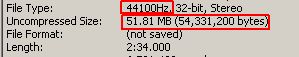
waveform properties like sample rate
The following are the waveform properties shown:
9.) Sample rate – in the above screenshot, the sample rate is 44100Hz. When recording/tracking, the most recommended sample rate should be greater than 44100Hz. Common values are 48 KHz, 88.1 KHz, 96 KHz and 192 KHz.
10.) Uncompressed size – this is the file size of the WAV file.
The last important property is the frequency characteristics of the digital audio waveform which you can see by doing a frequency spectrum analysis plot of the waveform. This will convert the time domain function (amplitude vs. time) to (amplitude vs. frequency). See the equivalent waveform in frequency domain:
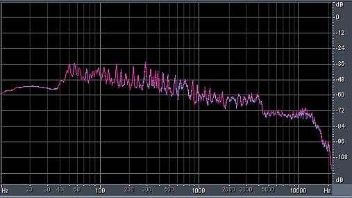
frequency domain plot
Thus it shows that below 40Hz, there is less energy as compared to 50Hz and 500Hz (where most energy is concentrated). There is also less mid frequency content from 1000Hz to 3000Hz and even lesser high-frequency energy. These frequency characteristics will be used by engineers to confirm the frequency content of the signal in relation to any EQ implementation.
Content last updated on August 8, 2012